Observability#
A service provider’s core router had a fan module fail silently overnight. There were no alerts. The thermal management subsystem on the line cards detected rising temperatures and began throttling the forwarding ASICs to protect the hardware. Throughput on a production transit link dropped by 40%. The monitoring system saw nothing: the thermal sensors it polled were on the chassis supervisor, not on the individual line cards. The SNMP polls ran every five minutes and reported the device as healthy. The interface counters showed reduced throughput, but no threshold was configured for that pattern because the link had always been well below capacity.
Three hours later, a customer SLA breach triggered a ticket. The on-call engineer SSHed into the router, noticed the fan failure in the local alarm log, and power-cycled the fan module. The fan controller restarted and thermal throttling lifted within minutes. Traffic recovered. The SLA breach was documented, the customer was notified, and the incident was closed.
The root cause was never confirmed. By the time anyone investigated, the router had been running normally for hours. There was no thermal data for the line cards, no record of the throttling event, and no way to correlate the throughput reduction with the fan failure in any monitoring system. The incident report concluded: “suspected hardware issue, resolved by hardware reset.” It happened again six months later on a different router.
The failure was not a missing threshold. The team had thousands of thresholds. The failure was incomplete coverage: the monitoring system collected from the sources that had always been polled, not from every source that could change device behavior. Thermal data from line cards was available via gNMI on all three chassis types in the fleet. Nobody had configured the collection path because nobody had written a runbook for fan failures.
Traditional network monitoring watches for broken things: is the interface up? Is the CPU over 90%? Is this service responding? That’s useful, but it’s reactive: you’re watching for failure.
Observability is different. It’s about understanding why things break or are about to break. It’s not just “that device is down” but “why is it down, what breaks because it’s down, what’s the business impact.” With network automation, observability becomes the feedback loop: you observe something, your system detects it, decides how to respond, takes action, and verifies the fix worked. That is a self-healing network, and Chapter 17 covers how to build one.
This chapter covers everything you need to see what’s happening in your network: what data to collect, how to collect it, how to store it, how to alert on it, and how to show it to people in a way that actually helps them make decisions. It also covers the part most teams skip, watching the automation system itself, which is where failures go silent.
We cover two building blocks here: Collector and Observability, because they’re tightly connected.
This chapter is heavily influenced by the book Modern Network Observability by Packt, that I coauthored with David Flores and Josh Vanderaa. If you want to go hands-on and learn an implementation with the TPG (Telegraf-Prometheus-Grafana) stack and other tools, I definitely recommend it.
Whether you use a traditional all-in-one platform (e.g., SolarWinds, LibreNMS), a cloud service (e.g., Datadog, New Relic), or build your own stack from open-source pieces (e.g., Prometheus, Grafana, etc.), the underlying architecture is the same. Understanding those patterns helps you choose the right approach for your scale and your team.
The vendors and products named in this chapter are examples, not recommendations. They illustrate a category; the right choice for your network depends on the factors this chapter works through.
Before going into the lower level details, here we establish the fundamentals of network observability within the network automation strategy, defining its goals and scope.
Fundamentals#
You can’t manage what you can’t measure.
You probably already monitor your network. You use Simple Network Management Protocol (SNMP), you look at System Logging Protocol (Syslog), you have dashboards showing link utilization. That’s monitoring: it tells you if things are working.
But automation needs more. When your network changes (maybe because automation changed it), you need to know immediately if it breaks something. When you get an alert, you need context: which customers does this affect? Which services failed? What’s the blast radius? Traditional monitoring gives you alarms. Automation needs intelligence.
Here’s the key difference:
- Monitoring: Is the interface up? Is the CPU high? Simple yes/no questions.
- Observability: Why did the interface go down? What’s it impacting? How do we fix it automatically? What happened historically that led to this?
Observability feeds automation. Your system observes the network, detects problems, decides what to do, takes action, and verifies the fix worked. That cycle repeating is called closed-loop automation, the subject of Chapter 16.
Traditional monitoring tools (the big monolithic ones like SolarWinds) try to do everything in one product. You can make that work, but you’re often paying for features you don’t need and constrained by features you do. The alternative is building observability from pieces: pick the collector that works for your devices, the storage that scales with your data, the alerting that fits your automation workflows. This is harder to assemble but much more flexible.
This chapter walks through both approaches and the patterns that work regardless of which you choose.
One initial choice is about how the platform runs:
Monolithic (SolarWinds, LibreNMS): One product does everything. You install it, configure it, and go. Good if your network is straightforward and you don’t have DevOps experience. Bad if you want flexibility or your network is unusual: you’re stuck with their model.
Cloud SaaS (Datadog, New Relic, Kentik): They run everything for you. Fast to deploy, no infrastructure headaches, beautiful dashboards out of the box. But you’re paying monthly based on volume, your data lives on their servers (matters for some compliance regimes), and when you hit their limits, you’re stuck. I’ve seen teams spend $50K/month on observability SaaS wondering why their CFO is unhappy.
Build-it-yourself (Prometheus + Grafana, or Telegraf-Prometheus-Grafana (TPG) stack): Total flexibility, no vendor lock-in, better economics at scale. But you’re now running databases, message queues, and collector infrastructure. If you don’t have people who can operate this stuff, you’ll spend more time fixing observability than fixing your network.
The real question: Do you have the team to run it? If yes, build it. If no, buy it. Don’t fool yourself about which category you’re in.
After that choice, two more questions come up:
- Where does it run? On your premises (you control everything, but you run it), in the cloud (they run it, but your data leaves your network), or hybrid (some places local, some places cloud)?
- What’s the cost model? Per device? Per metric ingested? Flat subscription? These decisions add up fast when you’re collecting millions of data points per minute.
Evolving from what you already run
Nobody starts from nothing. You have an Network Management System (NMS), years of SNMP polling, a wall of thresholds somebody tuned years ago, and a NOC trained on one specific console. The architecture in this chapter is the destination, not the first step, and the migration is where the risk actually lives.
Run both for a while. The old system keeps alerting while the new pipeline earns trust, and a parallel period of a few months is normal rather than a planning failure. What keeps it finite is deciding up front what “earned” means: the new pipeline catches the same incidents, with fewer false positives, over a defined window.
Move in this order, because each step makes the next one cheaper:
- Inventory first. Point the new collection at the Source of Truth instead of a hand-maintained list. Even if nothing else changes yet, you stop missing new devices.
- One data type, one use case. Interface counters for capacity, or BGP session state for one service. A narrow slice proves the whole pipeline end to end: collection, normalization, storage, alerting, dashboard.
- The alerts that actually page people. Port the rules that wake somebody up, not the four thousand that never fire. Most thresholds in an old system have never fired or never been acted on, and migration is the cheapest moment to delete them.
- The long tail, or never. Some of what the old system does is needed once a quarter. Leaving it there for another year is a legitimate decision.
The old system gets switched off when nobody has looked at it for a month, not when the project plan says so.
The observability system needs to solve several things:
Observe everything automatically. New device connects? It should start reporting data without someone manually registering it. New service comes online? It’s already being watched. This requires integration with your source of truth so observability knows what exists.
Handle heterogeneous environments with good data. Your network probably has Cisco, Arista, Juniper, cloud providers, Linux servers, containers. Each one has different ways to expose data. And forget 5-minute intervals: you need near-real-time data when automation is making changes.
Correlate data across layers. A server is slow. Is the network congested, or is it a database issue? You need data from network devices, servers, applications, all speaking the same language so you can draw lines between them.
Scale without melting. Networks grow. When you’re collecting a million metrics per second, traditional architectures crumble. You need systems designed for scale from day one.
Let people analyze the data intelligently. Give analysts access to query your data, not just pre-built dashboards, but powerful queries so they can answer their own questions. And they need both real-time data and history (trends, anomaly detection).
Detect problems and trigger the fix automatically. Most of the time, your automation should respond to issues without waiting for a human. Only when automation can’t figure it out should someone get paged. And that alert better explain what’s wrong, not just show raw numbers.
Show people what they need to see. A dashboard is worthless if it shows too much or the wrong stuff. Give the network ops team their view, the business their view, the engineers their view. Each person gets what helps them do their job.
Finally, before detailing the seven functionalities that make possible these goals, let’s clarify what falls within Observability’s scope.
What’s in scope
Observability explains what the network is doing. It does not decide what the network should be, and it does not change it.
The block owns observed state: the record of what the network is actually doing, along the whole path from a counter on a device to a dashboard somebody acts on. Collection, normalization, distribution, storage, analysis, alerting, and the views on top. Three parts of that are easy to overlook:
- Observation at several levels, so the same underlying data answers a technical, an operational, and a business question.
- Feedback into CI/CD pipelines, so automated testing and post-change validation have real data to check against.
- Observability of the automation system itself: the Collectors, processors, and alerting are production services, and they need monitoring like any other.
What’s out of scope
- Defining network intent: What the network should look like (Intent/SoT responsibility)
- Executing network changes: Actually implementing remediation (Executor responsibility)
- Orchestrating workflows: Coordinating multi-step remediation across multiple systems (Orchestrator responsibility)
This clear boundary ensures Observability focuses on detection and insights, while other building blocks handle intent definition, execution, and orchestration.
Transitioning to modern observability requires careful planning. Do not take it as something as simple as replacing one monitoring tool with another; you have to transform your mindset. With more power comes more responsibility, and you will have more to choose and adjust.
With the key concepts of the Observability block in place, let’s take each functionality in turn.
Functionalities#
Seven functionalities deliver those seven goals, one each. That one-to-one mapping, shown in Figure 7.1, is what connects a requirement to the component responsible for satisfying it.
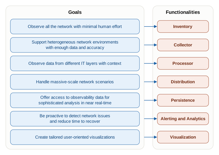
Inventory: Knows what to observe. It consumes intent from the SoT (devices, services, credential references) and hands every downstream component its targets and metadata. Add a device to the SoT and its monitoring comes online without anyone registering it.
Collector: Retrieves observed data from the network, both pull-based (polling) and push-based (streaming). SNMP for older equipment, gRPC Network Management Interface (gNMI) streaming for modern devices, Syslog for events, flows (NetFlow, IP Flow Information Export (IPFIX)) for traffic, packet captures for deep troubleshooting. Different speeds, different richness, and you do not have to pick just one.
Processor: Normalizes heterogeneous data into one schema and enriches it with context. One vendor’s metrics look nothing like another’s, logs arrive as unstructured text, and flows arrive as binary. The processor translates all of it into a common language and attaches which device, which customer, and which service each value belongs to.
Distribution: Moves data and events reliably from Collectors through processors to persistence and alerting. A sequential pipeline becomes the bottleneck at scale, so this is where message buses and streaming platforms decouple each stage and let them scale independently.
Persistence: Stores the normalized data where it can be ingested, retained, and queried at scale. Metrics want a time-series database, logs want something else, and both have to answer queries across millions of points in milliseconds. Not all databases are equal here.
Alerting and Analytics: Turns data into action. Raw metrics trigger nothing on their own, so rules and thresholds detect the conditions you care about and emit events: if CPU is over 90%, check whether a maintenance window explains it, and if not, hand the event to the Orchestrator or page someone.
Visualization: Renders the data and the events into dashboards and reports, tailored per audience. Data nobody looks at is wasted, and a dashboard that shows everything shows nothing: each audience gets the view that answers its own questions, able to drill down and to compare against history.
The functionalities can be seen in the form of a data pipeline, or Extract, Transform, Load (ETL), with this architectural view:
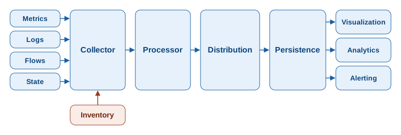
Those two figures are the map for the rest of the chapter. Each functionality gets its own section, in pipeline order, starting with the one that handles no observed data at all: working out what to observe in the first place.
Inventory#
The first question for the Observability block is what should be monitored.
You already have this data somewhere: it’s the inventory in your source of truth. You’ve got device names, service identifiers, IP addresses, what they are, whether they’re active, credentials. Don’t duplicate that by hand. Pull it in automatically.
What you need from your SoT:
- A unique name or ID for each device or service (so you know it’s the device you think it is)
- How to reach it: IP address, hostname, and credentials (if you need to actively pull data from it)
- What it is: the type and vendor (so you know which Collectors work with it)
- Whether it’s active: if it’s planned, active, or being decommissioned (so you don’t alert on expected downtime)
Beyond the basics, you might also care about:
- OS or device specifics: some devices use different protocols, some are old and need special handling
- Context: who owns it, where’s it located, which customers depend on it (useful for filtering alerts and dashboards)
Why automate this instead of building a list by hand? Because people forget to update lists. Devices get added, nobody tells monitoring, and suddenly you’re missing visibility. But if observability reads from your SoT, when you add a device there, it’s automatically being monitored.
To get this inventory data, you have two basic patterns:
- Pull: Observability checks the SoT periodically for updates. Simple, but if something changes mid-interval, you miss it.
- Push: When the SoT changes, it signals observability automatically (webhooks, message bus). Faster and more reliable, but usually a bit more complex because you need adjustments on both sides.
A third pattern sits between those two: a dynamic inventory service such as Consul or etcd. The SoT writes targets into a key-value store, each collector watches the keys it cares about, and a change reaches the collectors in seconds without either side knowing about the other. Prometheus-style service discovery reads this kind of store directly, which is why it is the common pattern in container-era stacks, but totally applicable to common networks too. It buys a network team two things: collectors can restart or scale out without re-reading the whole SoT, and a collector that loses the store keeps running on its last known target list.
If you have good data in your SoT and real integration (not manual copy-paste), inventory becomes automatic and you never miss observing a new device.
After the targets are defined, it’s time to collect operational data.
Collector#
Your data has to come from somewhere. Collectors are the bridges between your network and your Observability platform. They’re responsible for pulling (or receiving) data from your devices and feeding it into the pipeline. Without effective collectors, everything downstream is garbage.
There are two fundamental approaches from the perspective of who owns the data flow:
- Passive or Push: Your devices send data to the collector. Think syslog servers receiving log messages from routers, or IPFIX collectors listening for flow records. The device decides what to send and when.
- Active or Poll: The Collector asks devices for data. It connects to each device and pulls information using SNMP, gNMI, or Representational State Transfer (REST) Application Programming Interface (API)s. The collector is in control: it decides what to ask for and when.
Dial-in streaming sits across both. The collector initiates the subscription, then the device pushes until it is told to stop, so neither bullet describes it on its own. The streaming telemetry pattern below covers it.
You can also categorize collectors by deployment style:
- Agentless: No software to install on devices. A central collector server (usually running somewhere else) connects to each device individually. Simple to start with, but can become a bottleneck as you scale.
- Agent-based: Install a small agent on each device or service. Agents push data to a central location, or pull directly from local sources. More distributed, easier to scale, but more moving parts to manage.
Regardless of the collection method, it’s important to highlight the different types of data that may be of interest in the network automation environment. I classify it in four broad categories, shown in Figure 7.3:
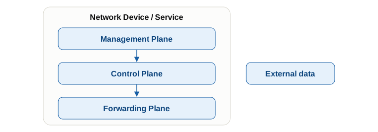
- Management plane: The state of the device, or to read data about the configuration, logging, or network statistics. Protocols in this group are SNMP, Syslog, gNMI, NETCONF, and RESTCONF.
- Control plane: This is where the distributed protocols that determine the packet forwarding of the network, such as layer 2 or layer 3 forwarding tables, run. A few examples of control plane protocols are OSPF, IS-IS, and BGP. This plane can be observed with techniques such as Ping or Traceroute, or telemetry protocols such as BGP Monitoring Protocol (BMP).
- Forwarding plane: This plane is where the packets are moved (e.g., network interfaces), and it is the most demanding in terms of data volume and velocity. Naturally, when observing it, it’s also crucial to not impact the primary goal of the plane, which is to forward packets. In this group, we have tools such as tcpdump, IPFIX, sFlow, NetFlow, IP SLA, PSAMP, and Extended Berkeley Packet Filter (eBPF).
- External data: This category includes everything that is not network device-specific. For instance, circuit provider information and the contact for a given interface, coming from an external asset manager system or physical Internet of Things (IoT) sensors, could fit into this broad field.
Observation is not free on the device. Every poll and every subscription costs the device something, and the budget you are spending is the control plane you are trying to protect. Walking a large routing or ARP table can pin a supervisor CPU for the duration of the walk. A subscription at 100ms consumes memory and processing on the box for as long as it runs. Even a steady 48 ports by 8 metrics every 30 seconds is load the device feels when nothing is wrong at all.
Treat collection as traffic you are adding to a production system: measure device CPU before and after enabling a new collection path, stagger polling so hundreds of devices are not answering in the same second, and take sub-second data from the handful of interfaces that need it rather than from the whole fleet. The failure mode is specific and familiar, which is monitoring that causes the incident it was installed to detect.
And it is not free on the network either. Telemetry is traffic, and it is heaviest exactly when something is wrong and everything reports at once. Two consequences follow. Prefer an out-of-band management network for collection wherever you have one: it keeps telemetry off the data path, and it is the only way an alert about a congested fabric escapes the congested fabric. And at high volume, consider a network dedicated to telemetry, or at minimum a Quality of Service (QoS) class for it, so the data describing an outage is not the first thing dropped during one. Where everything shares a single path, say so explicitly in the design and accept that your observability degrades along with the network it is watching.
These four categories end up mapping to two core questions:
- What to collect: Metrics? Logs? Flow records? Each has different data models. SNMP has MIBs, modern gear speaks gNMI, applications use OpenTelemetry. The dream is a universal standard that lets you correlate data across everything, but that doesn’t exist yet. So you might need to build your own translation layer that turns all these different formats into something consistent (which is what the processing layer does next).
- How to get it: Which protocol? SNMP is old but stable, gNMI is modern and pushes data at you continuously, IPFIX captures what’s actually flowing. It varies by what you’re trying to observe.
This table summarizes what you might collect and the tools available:
| Data Type | Protocols / Collection Methods | Notes / Examples |
|---|---|---|
| Metrics | SNMP, HTTP and CLI scraping, OpenTelemetry (OTLP), Streaming telemetry (gNMI) | Device metrics, host metrics, application metrics |
| Logs | OpenTelemetry (OTLP), file tailing, syslog | Application logs, system logs, structured logs |
| Traces | OpenTelemetry (OTLP) | Distributed tracing across services |
| Network Flows | NetFlow, IPFIX | Traffic flows, source/destination analysis |
| Protocol-specific | BMP, BGP, ARP, OSPF | BGP monitoring (BMP), ARP tables, BGP tables, OSPF tables |
| Packet Captures | PCAP (libpcap), SPAN / TAP | Full packet inspection, deep troubleshooting |
To get a deeper understanding of the different options, refer to the Modern Network Observability book.
CLI scraping is fragile (vendors change output format), slow (screen scraping and parsing text is expensive), unreliable (random command timeouts), and scales terribly. If your device is so old it only has CLI, either replace it or accept that you’ll have limited observability. Don’t build your entire monitoring stack around the lowest common denominator.
Network data collection applies to data centers, ISP backbones, cloud network services, Linux kernel interfaces, or raw packets. It depends on your environment.
Here’s the key: before you decide what to collect, start with the problem you’re trying to solve. That decision drives everything else. Are you detecting interface saturation? Monitoring BGP convergence? Tracking DDoS traffic? Your problem determines what data you need and how often you need it.
To increase the frequency of data collected (interesting in some cases) or to converge collection methods, these are a few patterns that have increased adoption recently:
Streaming telemetry
Devices push data continuously using YANG models. You set up subscriptions and data flows in real-time. It comes in two flavors, shown in Figure 7.4:
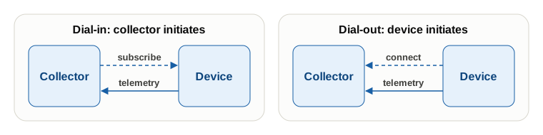
- Dial-In: Collector asks device to start streaming (collector initiates).
- Dial-Out: Device is pre-configured to stream to you (device initiates).
Much lower latency than polling, and the device stays in control of the flow.
Not every protocol that can stream does it the same way, and the differences decide how you design subscriptions:
- gNMI defines the subscription model most network engineers mean by streaming telemetry. A subscription runs in one of three modes:
ONCE(one set of updates, then the RPC closes),POLL(a long-lived RPC where the client asks when it wants data), andSTREAM(long-lived, the target keeps sending). Inside aSTREAMsubscription, each path choosesSAMPLE(one update per sample interval),ON_CHANGE(an update only when the value changes), orTARGET_DEFINED(the device decides per leaf). - NETCONF with YANG-Push is the IETF equivalent. RFC 8639 defines subscriptions to YANG notifications and RFC 8641 extends them to datastore updates, with the same two triggers, periodic and on-change, plus a dampening period that bounds how often an on-change subscription may fire.
- OpenTelemetry Protocol (OTLP) is not a device subscription mechanism at all. It is how an agent or collector pushes telemetry it has already gathered, which places it downstream of the two above rather than in competition with them.
- Flow and event exports (IPFIX, sFlow, BMP, Syslog) are push by nature. There is no subscription to negotiate: you configure the device to send, and the collector listens.
One thing to know before you design around the figure above: dial-out is not part of the gNMI specification. The spec defines dial-in and lists dial-out as a future item, so every dial-out implementation you meet is vendor-specific. Instead of adding a dial-out mode to gNMI, OpenConfig defined a generic gRPC tunnel. Check what your platforms actually support rather than assuming the pattern is portable.
Within the streaming telemetry realm, push the sample interval far enough down and it answers a question polling cannot reach at all. This is what High-frequency telemetry (HFT) is about. A microburst is a traffic spike lasting between ten milliseconds and a second: long enough to fill a queue and drop packets, short enough that a five-minute average still shows the link at 30% utilization. The customer sees loss, the dashboard shows headroom, and the argument that follows is familiar to anyone who has run a data center fabric.
Catching it takes one of two things. Either a sub-second sample interval, with 100ms a common choice, or hardware-level export from the ASIC, where the switch records queue depth at a granularity no subscription could carry. Both have become ordinary requirements in AI training fabrics, where incast from synchronized workers is the normal traffic pattern rather than the exception.
The cost is volume, and it is not subtle: moving from a 5-second to a 100ms interval multiplies the data by 50. So high-frequency telemetry is almost always paired with filtering at the collector and aggregation close to the device, both covered later in this section. Sample at 100ms on the interfaces where microbursts matter, not on all of them. And, as the Persistence section covers, use downsampling for long-term analysis.
Hypertext Transfer Protocol (HTTP)-exposed metrics
HTTP scraping (pull-based metrics) is simple and scales well. SNMP works this way too, but the interesting development is narrower than it is often described: Linux-based network OSes let you run a Prometheus exporter on the switch itself. Metrics then arrive over HTTP, in a format your systems-monitoring stack already speaks, with no Management Information Base (MIB) parsing in between.
| Source | Exposed by | Example metric (interface traffic) |
|---|---|---|
| SONiC | sonic-exporter, running on the switch | sonic_interface_receive_bytes_total{device="Ethernet0"} 1.234e+12 |
| NVIDIA Cumulus Linux | node_exporter, running on the switch like on any Debian host | node_network_receive_bytes_total{device="swp1"} 9.21e+10 |
| Arista DANZ Monitoring Fabric | the DMF controller, on /api/v1/metrics/prometheus, not the switch OS | device_interface_in_octets_total |
Note the third row. Arista EOS has no on-box Prometheus endpoint of its own, so the way to Prometheus-format data from EOS is a collector pointed at gNMI, which is the streaming telemetry pattern above. Check what your own platforms actually expose before designing around this, because the gap between “the NOS is Linux” and “the NOS ships an exporter” is where plans go wrong.
HTTP-exposed metrics make life much easier for the many infrastructure teams that already converge systems monitoring on Prometheus, because network data arrives in a format their stack already speaks.
The scraping approach provides low latency and near-real-time metrics, rich labels, and pull-based collection (central control of rate/timeout), connecting well with cloud-scale observability.
OpenTelemetry
OpenTelemetry is a vendor-neutral standard and toolkit for collecting, processing, and exporting telemetry data. Think of it as a common telemetry language and pipeline that unifies metrics, logs, and traces across networks, systems, and applications.
It does not replace network protocols like SNMP, NetFlow, gNMI, or BMP. Instead, it standardizes how telemetry is represented and transported after collection.
In traditional network monitoring, the data models are diverse and use vendor-specific schemas and naming, which makes it hard to correlate across layers (network ↔ system ↔ application). In contrast, OpenTelemetry helps by providing:
- A common data model for metrics, logs, and traces
- A standard transport protocol (OTLP), over gRPC Remote Procedure Call (gRPC) or HTTP
- A single processing pipeline for multiple signal types
The network side of OpenTelemetry is still being written. The semantic conventions for network hardware metrics define names such as
hw.network.io,hw.network.packets, andhw.network.bandwidth.utilization, but every one of them is still marked Development rather than stable. Treat them as a direction of travel rather than a contract: the names can still change, and almost no network device emits them natively today.
The reference implementation is the OpenTelemetry Collector, which receives, processes, and exports telemetry in a vendor-neutral way. Grafana Alloy and Telegraf are alternatives that speak OTLP alongside their own ecosystems. All three collect from different exporters and write to different backends: metrics into Prometheus-compatible Time Series Database (TSDB)s, logs into Loki, Elasticsearch or ClickHouse, and traces into Tempo or Jaeger.
Adopting OpenTelemetry is not just a tooling decision: it is an architectural decision about how you unify your observability pipeline. The choice is between two approaches:
Protocol-native: each signal type travels through its native protocol end to end (gNMI to Prometheus, syslog to Elasticsearch, NetFlow to ClickHouse). Each pipeline is optimized for its signal. The cost is multiple independent pipelines with no shared data model, making correlation across signal types expensive.
OTel-native: signals are converted to OTLP as early as possible and flow through a single pipeline to a unified backend. Correlation across metrics, logs, and traces is natural because they share a data model. The cost is that network device OTel support is still maturing: most vendors do not emit OTLP natively, requiring an adapter layer (gNMI to OTel, SNMP to OTel) that adds operational complexity.
The practical recommendation for network automation environments today: adopt OTel for application-adjacent signals where vendor support is strong (automation platform telemetry, service health, structured application logs) and continue with protocol-native pipelines for traditional network telemetry (SNMP polling, gNMI streaming) until device-side OTel support matures. Design the pipeline to accommodate both approaches side by side rather than forcing a premature standardization that requires adapters for every network device.
The trend is clear: OpenTelemetry will eventually become the standard for all observability data. Starting with it for the automation platform itself, the meta-monitoring covered later in this chapter, is a low-risk first step that builds familiarity before extending it to network devices.
And this brings us to a final consideration about the common structure of modern pluggable collectors, with Input, Processor and Output stages.
Collector Architecture
Simplistically, every collector can be broken down into three parts (sometimes these are pluggable and others are more hardcoded).
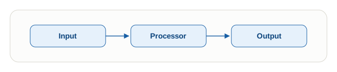
- Input: It defines what has to be observed and under which parameters.
- Processor: Even though it is optional, it’s very convenient as soon as data enters the data pipeline to ensure data structure consistency. The processing could become very complex and may impact performance at scale, so not all processing has to be done at this level (more about this in the next section).
- Output: Defines how the collector moves the data into the pipeline. It may send it directly to other blocks like processing or persistency, or use the distribution component to scale.
There are many collectors (each one with different capabilities) such as Telegraf, Grafana Alloy, gNMIc, PMACCT, goflow, etc., but they use a similar architecture. So when choosing one, and sometimes you need several, weigh four things:
- Device capabilities, what protocols do your devices support?
- Data volume, high-volume needs streaming; low-volume can use polling.
- Latency requirements, near real-time vs. traditional intervals.
- Team skills and ecosystem fit with your backend.
Where to start, if you are starting now. Everything above is a catalogue, not a to-do list. Start from the most capable thing each platform actually supports and work down, rather than starting at the common denominator:
- Streaming telemetry wherever it exists. A gNMI subscription, YANG-Push over NETCONF, or an on-box exporter scraped over HTTP all give you structured data, on-change semantics, and intervals measured in seconds instead of minutes.
- Flow export when you need to know who uses the capacity. “Who is using this capacity” is a different question from “how much is being used”, and no interface counter answers it.
- SNMP only for the devices that offer nothing better. It is a compatibility floor rather than a design choice. Building the pipeline around it means designing for your weakest input and retrofitting everything else later.
- CLI scraping as the last resort. At that point you are really choosing between a hardware refresh and accepting that part of the fleet stays dark.
Everything else on the list, packet capture, eBPF, sub-second telemetry, is a specialized answer to a specialized question: adopt it when you have the question, not because it appeared in this chapter.
The “complete” network observability solutions, such as Suzieq and Kentik, implement built-in collectors for the data they cover.
The collector’s own processing stage introduces the next functionality: the Processor, which manipulates data at several points in the pipeline.
Processor#
Raw data from collectors is messy. Different devices export metrics differently, logs are unstructured text, values might be in different units. The processor layer cleans this up and makes it useful.
Goal: Once data is received, it must adhere to shared standards in order to converge signals from multiple sources, correlate them, and enrich them with additional context. Without this processor step, observability pipelines quickly become fragmented, difficult to query, and expensive to operate. There are multiple opportunities to process it depending on scale, complexity, and operational requirements.
These processors may be run at different stages of the observability pipeline, depending on the use case:
- Embedded in the Collector: Best for lightweight, early normalization and filtering
- Dedicated processor: Required at scale for dynamic enrichment and complex transformations
- Persistence layer: Suitable for recording rules and long-term rollups (Normalization should always happen before this)
- Alerting layer: Derives events from stored data and applies business logic
The following are common processing actions that apply to observability pipelines.
Normalization#
Data comes in different formats. One vendor’s metrics look nothing like another’s, syslog is text, NetFlow is binary. Normalization translates all of this into a common format so your backend doesn’t have to understand 50 different dialects.
Within normalization, those actions come down to two: enforcing a data structure, and renaming and aligning what the sources call things.
There is a third alignment that is easy to forget, and it is time. Every correlation in this chapter assumes a timestamp from one device means the same instant as a timestamp from another. That holds only if the fleet is synchronized and the pipeline is explicit about which clock it trusts. Keep Network Time Protocol (NTP) healthy and monitored, store everything in UTC, and decide whether a record carries the device’s timestamp or the collector’s, because the two differ by the collection delay and mixing them silently skews every comparison you make later. A device whose clock has drifted by two minutes raises no error. It produces a correlation that is quietly wrong.
Structuring
Devices emit data in ways that make sense for them. Your job is to translate that into a format that works for analysis. For example:
Log-based: parsing unstructured text into structured data.
Mar 18 14:22:11 leaf01 IFACE-5-STATE: swp1 oper-state changed from UP to DOWNto
{ "timestamp": "2025-03-18T14:22:11Z", "level": "INFO", "device": "leaf01", "component": "interface", "event": "oper_state_change", "interface": "swp1", "previous_state": "UP", "current_state": "DOWN" }Metric-based: enforcing a consistent syntax:
<metric name>{<labels>} <value>interface_admin_state{hostname="leaf01", ifname="swp1"} 1 interface_oper_state{hostname="leaf01", ifname="swp1"} 0 interface_speed_bps{hostname="leaf01", ifname="swp1"} 100000000000 interface_in_errors_total{hostname="leaf01", ifname="swp1"} 0 interface_out_errors_total{hostname="leaf01", ifname="swp1"} 12Table-based: some tools (e.g., Suzieq) organize data into tabular, time-indexed state views:
| hostname | ifname | adminState | operState | speed | inErrors | outErrors |
|----------|--------|------------|-----------|-------|----------|-----------|
| leaf01   | swp1   | up         | up        | 100G  | 0        | 0         |
| leaf01   | swp1   | up         | down      | 100G  | 0        | 12        |
Renaming and alignment: Different telemetry sources describe the same concept using different names, paths, and label conventions or values. For example, the same naming for operational status:
- Openconfig: /interfaces/interface/state/oper-status value: UP tags: source=192.0.2.1 and interface_name=eth1
- SNMP: ifOperStatus{ifName="GigabitEthernet0/1", device="router01"} 1
- Native Prometheus: interface_oper_state{interface="swp1", host="leaf01"} 1Normalization aligns them into a consistent model, including the object name, label renaming, and the value (using the same unit conversion):
intf_oper_state{name="eth1", device="192.0.2.1"} 1
intf_oper_state{name="GigabitEthernet0/1", device="router01"} 1
intf_oper_state{name="swp1", device="leaf01"} 1Enrichment#
Enrichment adds extra content to the observability data beyond what is actually observed. These extra dimensions allow more sophisticated data consumption. For example, you may be able to understand that the metrics belong to a device that plays a specific role in the network and act accordingly.
There are two main approaches to enrichment:
Extending data: Adding extra metadata or labels to the observed data to complement it. This data could be static (e.g.,
org=my-company) to mark all your data, dynamic based on collection context (e.g.,collector_id=1234), or dynamic based on the observed data itself (e.g., givenhostname=rtr-1, create a labellocation=BCN01by correlating with the SoT).intf_oper_state{ name="swp1", device="leaf01", role="leaf", location="BCN01" } 1Creating new data: Following the Prometheus ecosystem’s “info metrics” pattern, we can generate metrics that carry no measurement at all, only context data about the object. These metrics are useful in later observability pipeline stages to add more dimensions to analysis, as you will discover in the Alerting section.
device_info{
    name="leaf01",
    role="leaf",
    vendor="arista",
    model="7050SX3",
    platform="eos",
    os_version="4.29.2F",
    location="BCN01",
    rack="AB1",
    rack_unit="U32",
    environment="prod"
} 1
The info metrics are a curious type of data that do not have the relevant data in the value (e.g., the 1 in the previous metrics) but in the labels. This trick allows reusing TSDB that do not support some type of values (like strings).
Both approaches add labels and context. That’s powerful for alerts and analysis. But there’s a cost to think about:
- Cardinality: Every new label multiplies your time series. Device × interfaces × metrics is already high-cardinality. Add labels carelessly and storage explodes, queries slow down. Be thoughtful.
- Update frequency: Device racks and management IPs don’t change every second. Don’t poll enrichment data like you poll volatile metrics. Event-driven updates work better, fewer queries to your source of truth.
- Resilience: If your source of truth goes offline, enrichment stops. Cache it so you keep operating, even degraded. Your automation relies on this data, so make it rock-solid.
Transformation / Derivation / Aggregation#
Take raw metrics and derive new ones from them. Example: merge all interface input traffic from leaf and spine switches into a single “fabric bandwidth used” metric for trending. You’re combining existing data to answer bigger questions or feed dashboards. For example:
- record: fabric:interface:in_bps
expr:
    (
    sum by (fabric, role, hostname, name) (
        rate(interface_in_octets_total{role=~"leaf|spine"}[5m])
    ) * 8
    )
    * on (hostname, name) group_left (fabric, role)
sot_interface_info{role=~"leaf|spine"}In the Prometheus ecosystem, this is known as recording rules, but I prefer to call them composed metrics.
Composing metrics this way buys three things. Reusability: the fabric bandwidth metric is defined once, and every alert, dashboard, and report reads the same number, so nobody argues about whose query was right. One definition behind alerts and graphs: an alert that fires on fabric:interface:in_bps and a graph that plots it cannot disagree, which removes the whole class of incidents that start with “the alert says 80% but the dashboard says 60%”. Query performance: the expensive aggregation runs once per evaluation interval instead of once per dashboard refresh, which matters when it spans thousands of interfaces.
The cost is storage and one more thing to maintain. Every composed metric is persisted alongside the raw data it came from, and its definition has to be updated when the underlying labels change. So compose the metrics you query repeatedly, not everything you could.
Aggregation is the other way to reduce volume: drop dimensions you do not need for the question the data has to answer. Summarize interface counters per device, or device counters per site. Rate calculations from counters and histogram bucketing belong here too, and both are useful across a wide range of analyses.
Filtering#
Drop the junk early. Not every log line is worth storing. Not every interface metric matters (maybe you don’t care about loopbacks). The earlier you filter, the less you waste on storage and processing. Allowlists (only keep this) are safer than denylists (drop that).
Filtering starts in the subscription, not in the processor. Ask only for the paths you need, then drop whatever still gets through. With gNMIc, both halves are configuration:
subscriptions:
  interface-counters:
    paths:
      - /interfaces/interface/state/counters
    mode: sample
    sample-interval: 30s

processors:
  drop-loopbacks:
    event-drop:
      tags:
        - "^Loopback.*"

outputs:
  prom:
    type: prometheus
    event-processors:
- drop-loopbacksThe subscription stops the device sending anything but interface counters. The processor then drops the loopbacks, which no path filter can exclude because a loopback is an interface like any other. The order matters: the narrower the subscription, the less work every stage downstream has to do.
Sampling / Throttling#
Even after filtering, volume might still be too high. Throttle it. Sample probabilistically (“keep 10% of these flow records”), focus on top-K metrics (“only store the 100 busiest interfaces”), or rate-limit per source (“max 1000 metrics per device”). As data ages in your database, roll it up (5-second granularity becomes 5-minute averages) to save space.
A concrete shape for a 2,000-interface fabric: keep 100ms counters on the 40 uplinks that carry inter-rack traffic, 10-second counters on every access port, and nothing at all on administratively down ports. Then roll the 100ms series up to 10-second averages after 24 hours, and to 5-minute averages after 30 days. The uplinks keep the resolution that catches microbursts, and the storage bill reflects the 40 interfaces that needed it rather than all 2,000.
The same logic applies later in the pipeline, when you decide what to persist and what to drop.
In practice, effective observability pipelines distribute processing across layers, depending on tooling, scale, and operational constraints.
Distribution#
Simple linear pipelines (collector → processor → database) don’t scale well. If the database gets slow, the collector backs up. If you need to upgrade the processor, you stop collection. Everything is tightly coupled and fragile.
This is where message brokers come in.
Message brokers like Apache Kafka or NATS sit in the middle. Producers (collectors, devices) publish to topics. Consumers (processors, databases, alerting) pull at their own pace. Fully decoupled, which brings three benefits:
- Scaling: Each component scales independently.
- Resilience: If a consumer is slow, data queues up instead of being dropped.
- Flexibility: Same data feeds multiple backends without duplication at the source. Upgrade or restart one component without affecting others.
Think of it as a buffer that absorbs spikes gracefully.
See Chapter 12 for more on scaling and reliability patterns.
Hot and cold data
A message broker is not only a transport. It is also the one place in the pipeline where you can afford to keep everything. Figure 7.6 shows the shape: the full firehose lands in hot storage, and only two things move on to cold storage.
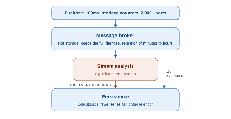
Think of it as hot storage: a short retention window, minutes or hours, holding the full firehose exactly as it arrived. Nothing in it is persisted in the sense the next section means, so volume costs you a retention setting rather than a storage bill. Cold storage is the opposite trade. The persistence layer keeps far less data for far longer, and every series you add there you pay for until its retention expires.
That difference is what makes stream analysis worth doing. 100ms interface counters across a 2,000-port fabric are too expensive to persist and perfectly affordable to pass through a broker, so you can run microburst detection against the stream and persist only what it finds: one event per burst instead of 20,000 samples a second. The data that produced the event is obsolete within the hour, and that is fine, because the event outlives it.
Persist a coarse sample alongside the event and you keep the trend without keeping the firehose. Ten-second or one-minute averages of the same counters cost a fraction of the raw series, and the two answer different questions: the event says a burst happened at 02:41:13 on this port, and the coarse series says whether bursts are becoming more frequent on that fabric. Neither is a substitute for the other, and together they are still far cheaper than persisting everything.
This is why Alerting and Analytics reads from both sides. Against cold storage it answers questions about trends and history. Against the hot stream it answers the questions that would be unaffordable to store, which is exactly where the volume lives.
Hot storage buys you a window. Anything that has to outlive it goes to the block that comes next.
Persistence#
Once data is processed, it needs to live somewhere. The database layer stores all your observability data. It needs to handle huge volumes, support fast queries, and keep costs reasonable.
Metrics, logs, flows and traces are the obvious contents, but two more kinds of data belong here, and both are easy to forget until an incident needs them:
Observed state: the structured record of what the network actually is. Which interfaces exist and what they are called, which neighbors each device really sees, which routes are installed, which VLANs are present on which trunk. This is the same shape as the model Chapter 4 describes for intent, holding the opposite content: not what the network should be, but what it is. Keeping it queryable is what lets you answer “which devices lost an OSPF neighbor between 02:00 and 02:10” without logging into anything, and it is what drift detection compares against intent. The familiar name for this category of tool is the Configuration Management Database (CMDB), and it belongs here rather than in the Source of Truth for the reason Chapter 5 gives: a CMDB records what is in the network, populated by discovery, while the SoT declares what should be.
Configuration backups: the running configuration of every device, captured on a schedule and on every change. In a post-incident investigation it is the only record of what the device was actually told to do.
A configuration backup store is a credential store whether you planned it or not. Device configurations carry hashed local passwords, SNMP communities, RADIUS and TACACS+ shared secrets, BGP MD5 keys, and tunnel pre-shared keys. Chapter 4 insists the SoT holds references rather than secrets, and the backup repository is where that discipline is most often lost. Give it the access controls, encryption, and audit trail you give the secrets manager, scrub what you can on ingest, and never let it become the convenient read-only copy everybody has access to.
Good databases for observability share common traits:
- Time-aware: Data is inherently timestamped. Databases optimize for range queries and time-windowed calculations.
- High write throughput: Constant metric ingest. Databases handle it without slowing down.
- Multi-dimensional: Metrics carry labels (device, interface, location). Query and aggregate them efficiently.
- Flexible queries: Need expressive languages (PromQL, LogQL) to explore data without predefined schemas.
- Lifecycle management: Storage grows fast. Support retention, downsampling, deletion to control costs.
- Schema flexibility: New metrics appear constantly. Databases handle evolution without costly migrations.
What database types work?
No single database handles all observability workloads perfectly, and anyone telling you otherwise is selling something. Here’s what actually works:
Time-series databases (TSDB): This is where you start. Prometheus won the metrics war. Its data model (metrics with labels) became the de-facto standard, and PromQL is the query language everyone knows.
Columnar databases: ClickHouse is the king here. It’s absurdly fast for log aggregation and flow analysis. If you need to query billions of rows for reporting or historical analysis, this is your tool. Parquet files work for analytics workloads where you don’t need real-time writes (like Suzieq does).
Text-search databases: for unstructured log search, Elasticsearch is the established option, and Loki takes a lighter approach by indexing labels rather than full text, which costs less to run at the price of slower arbitrary searches. Commercial platforms such as Splunk bring mature analytics. One point matters more than the product choice: most teams over-invest in log search and under-invest in structured logging, and structured events reduce how much free-text searching you need in the first place.
My recommendation: Start with Prometheus (or similar) for metrics, Loki (or similar) for logs. Add ClickHouse (or similar) when you need serious historical analysis. That stack will get you to massive scale before you need something fancier.
This classification is not absolute; most tools have a primary classification but then implement some characteristics of others (especially time-series).
Two important concepts when designing storage: cardinality (how many unique values can a label take) and dimensionality (how many labels does one metric have). High-cardinality labels multiplied by many dimensions = explosion in stored data and slow queries. This is one of the biggest challenges in observability. Chapter 12 covers the scaling side in depth.
Each database has its own characteristics that must be mapped to the use cases it needs to solve. For example, Suzieq uses a columnar solution (Apache Parquet files) because the questions it tries to answer are relational rather than time-series based. For example: “Which routes exist on spines but not on all leaves?” These questions require:
- Filter across many attributes
- Compare rows across devices
- Join tables (interfaces, neighbors, routes)
- Look at state at a point in time (not historical evolution)
This is what a columnar analytic solution is designed for. A TSDB could help with checking the number of routes, but to identify missing routes would require many labels, which is not its primary strength.
Downsampling is what makes long retention affordable. A counter sampled every 10 seconds produces 8,640 points per day per series; averaged to 5 minutes it produces 288. Keep both and you have answered two different questions: the raw data serves the incident you are debugging this week, and the rolled-up data serves the capacity plan you write next quarter.
| Stage | Resolution | Typical retention | What it answers |
|---|---|---|---|
| Raw | 10s or finer | 24 hours to 7 days | What happened during this incident |
| First rollup | 1 to 5 minutes | 30 to 90 days | Last month’s trend, post-incident review |
| Second rollup | 1 hour | 1 to 3 years | Capacity planning, year-on-year growth |
Two rules keep this honest. Decide what each stage is for before you set its retention, because “keep everything for a year” is a budget decision disguised as a technical one. And choose the aggregation per metric rather than globally: averaging a utilization gauge is reasonable, but averaging a peak is how you lose the microburst you spent the collection budget catching. Keep max alongside mean wherever the spike is the signal.
After all the data management, there are two final steps:
- Create events for other automation to use or humans to intervene: Alerting and Analytics
- Visualize the data to provide information for decision-making: Visualization
Alerting and Analytics#
Alerts turn data into action. Your goal: feed them to automation. Notify humans when automation can’t fix it.
Alerts flow through four stages, shown in Figure 7.7:

- Detection: Find something wrong in data.
- Processing: Enrich with context. Is it critical? Minor? False alarm? Correlate related alerts to reduce noise.
- Routing: Send to orchestration (run workflows), teams (Slack), or incident management (PagerDuty).
- Escalation: If automation fails, humans take over.
The hard part isn’t setting up alerts. It’s preventing alert fatigue. I’ve seen NOCs with 10,000 active alerts where nobody looks at any of them anymore. At that point, you don’t have monitoring, you have expensive noise.
Here’s how you actually fix it:
Route most alerts to automation, not humans. If a human sees an alert, it should be because automation tried and failed. Interface flapping? Automation checks if it’s maintenance, reboots the optics, opens a ticket with the vendor. A human only gets paged if automation can’t resolve it.
Remediation is automation like any other, and it needs the same protections: a dry run before the first real action, a blast-radius limit so one rule cannot touch the whole fleet, an approval gate for anything outside an agreed safe set, and a rollback path. Chapter 6 covers those controls and Chapter 8 covers who sequences them. An alert that triggers an unguarded change is worse than an alert nobody reads.
Kill static thresholds. “CPU > 80%” alerts are useless. 80% might be normal for that device. Use dynamic baselines: alert when something deviates from its historical pattern, not from some arbitrary number.
Group related alerts. When a core switch dies, you’ll get 500 alerts from downstream devices. Show one: “Core switch down, 500 devices affected.” Not 500 individual alerts.
Require a runbook for every alert. If you can’t write down what someone should do when they get the alert, delete the alert. Seriously. If the action is “investigate,” that’s not an action, that’s a waste of time.
Measure alert quality. Track false positive rates. Any alert with >10% false positives gets fixed or deleted. Track time-to-acknowledge. If alerts sit unacknowledged for hours, they’re not important enough to exist.
The goal is not “comprehensive monitoring.” The goal is “only page humans for things humans need to fix.”
The role of AI and AIOps in observability#
Let’s cut through the hype: most “AI-powered observability” is just anomaly detection with a marketing budget. That said, there’s real value here if you deploy it correctly.
What actually works:
Anomaly detection: ML is genuinely better than static thresholds at learning “normal” for each device. CPU at 85% might be fine for device A, disaster for device B. ML figures this out automatically. This is table stakes now, not magic.
Alert correlation: When 50 things break simultaneously, ML can group them and suggest “the core switch is probably the root cause.” Saves hours of troubleshooting. But you still need humans to verify, because it gets the root cause wrong often enough that acting on it unchecked will eventually take down something that was healthy.
Capacity forecasting: ML is decent at “based on trends, this link will saturate in 6 weeks.” Better than humans eyeballing graphs. Still needs human judgment on whether to care.
What’s oversold:
Automatic root cause analysis: Every vendor promises this. None deliver reliably. You’ll get suggestions, sometimes good ones, but “AI diagnosed and fixed the problem” is a demo claim, and the demos are chosen carefully.
Self-healing networks: Automation can fix known problems with known solutions. That’s not AI, that’s good engineering. True “self-healing” for novel problems doesn’t exist yet. When vendors demo it, ask them to show you the failure cases. Where that line actually sits, and how much you can build on the known-problem side of it, is the subject of Chapter 17.
“AIOps replaces your NOC”: No. AIOps helps your NOC be more effective. The human judgment, business context, and ability to handle edge cases? That’s still humans.
Bottom line: Use ML for anomaly detection and alert ranking. Be skeptical of everything else until you’ve tested it on your actual network, not a vendor demo.
Testing it is concrete work, not a feeling. Take 90 days of your own history, replay it through the tool, and answer three questions. Did it flag the incidents you actually had, and how much earlier than your existing thresholds? How often did it flag something that turned out to be nothing, counted per week per engineer, because that is the number that decides whether anyone keeps reading its output? And when it grouped alerts, was the cause it named the thing you actually fixed? A tool that beats your current thresholds on the first question and survives the second is worth turning on. One that cannot be measured against your own history is a demo, whatever the label on it says.
The alert-to-action interface#
An alert that a human reads is a notification. An alert that automation consumes is a contract. These two consumers have different requirements, and conflating them is one of the most common reasons alerting pipelines fail at the Orchestrator boundary.
When an alert is destined for automation, its payload must be machine-consumable without parsing. That means structured data, not a human-readable subject line. At minimum, an automation-destined alert payload should include:
- Device identity: a canonical identifier that matches the SoT record exactly (not a hostname that may differ between DNS and the CMDB).
- Alert class: a stable, enumerated type the Orchestrator can route on (not a free-text description that changes when someone edits the alert rule).
- Severity: a defined enumeration, not a numeric threshold value.
- Timestamp: the event time in UTC ISO 8601, not the notification delivery time.
- Relevant context: the specific metric or state that triggered the alert, in a field the Orchestrator can read directly (e.g.,
"interface": "Ethernet0/1", not embedded in the message string). - Source trace: a link or reference back to the raw event in the Observability system, so the Orchestrator can re-query for additional context.
A payload that meets this contract allows the Orchestrator to route the alert to the correct workflow, pass the device identity to the SoT lookup, and invoke the Executor with structured parameters, without any string parsing. A payload that does not meet this contract forces the Orchestrator to parse human-readable text, which breaks every time the alert description changes.
Define this contract before you build the alerting rules, not after. Alert rule authors who write for human readability produce messages that are hard to automate. Alert rule authors who write for both audiences produce messages that serve neither well. The cleanest solution is two parallel routing paths: one alert format for humans (Slack, PagerDuty), one for automation (message queue, webhook endpoint). Both triggered by the same detection rule; different payload templates for different consumers.
Alerts are what the system says when something needs doing. The last functionality covers what it shows when somebody wants to look.
Visualization#
All the observed data should provide value to the decision-makers, so user-oriented visualization has to answer their actual needs. That is the job of this final block: the dashboard and report layer.
Let me be blunt: most dashboards are terrible. They’re either vanity metrics that make executives feel good (“99.99% uptime!”) or they’re data vomit (50 graphs per screen, nobody knows what any of them mean).
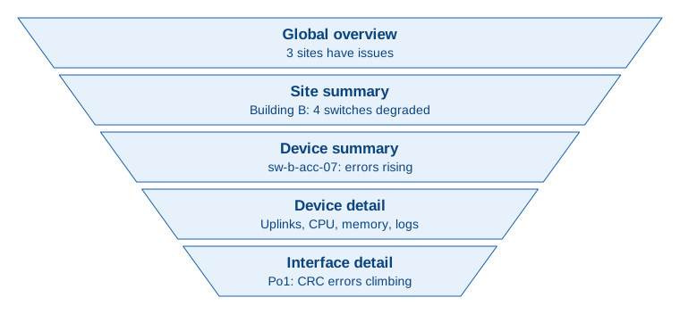
The principle that matters most is hierarchy, and Figure 7.8 shows the drill-down path it describes. Here’s how to build dashboards that actually help:
Relevance. Build for decisions, not decoration. Every widget should answer a specific question or trigger a specific action. If someone looks at a graph and doesn’t know what to do with it, delete the graph or redesign it.
Clarity. Show problems, not raw data. Green, yellow, and red signals beat numbers, and every element on the screen should have a purpose. “Interface utilization: 45%” is useless. “Interface utilization: normal”, or “WARNING, trending toward saturation”, is actionable.
Hierarchy. Drill-down beats one big dashboard. Start with a global health summary (“3 sites have issues”). Click a site to see device health. Click a device to see interfaces. Five focused dashboards beat one cluttered disaster.
Audience. Match the view to the reader. NOC staff need real-time operational status and drill-down. Managers need trend summaries and business impact. Engineers need raw data access and query interfaces. One dashboard trying to serve everyone serves no one.
Interactivity. Make it interactive or don’t bother. Static dashboards age badly. Let people filter, zoom, and adjust time ranges, so the dashboard supports investigation instead of just showing pictures.
And here’s the controversial take: most teams have too many dashboards. I’ve seen organizations with 200+ dashboards where each person looks at 2 of them. Delete the dashboards nobody uses. If no one looks at it for 3 months, it doesn’t matter.
The Visualization/Presentation boundary
Visualization sits at an architectural boundary that is worth addressing directly rather than leaving as a footnote. The Presentation layer (Chapter 9) is responsible for user-facing interfaces: access control, self-service portals, ITSM integration, and the user experience design of how people request and consume information. Visualization of observability data belongs here because the design decisions are driven entirely by the data: which metrics are available, how the alerting is structured, what drill-down paths the persistence layer supports. You cannot design an effective observability dashboard without understanding the data model behind it.
The distinction that matters in practice: dashboards built directly on observability data for operational decisions (what is happening right now, is this service healthy) are an Observability concern. How those same dashboards are surfaced to non-technical users, embedded in a self-service portal, or integrated with change management workflows is a Presentation concern. Chapter 9 revisits these tools from that access and workflow perspective. Most visualization tools (Grafana being the most common) blur this line by doing both, which is why the separation feels artificial. It is not. The concerns are genuinely different even when the same tool serves both.
In the Modern Network Observability book, chapter 11 (“Application of Your Observability Data”) you can find a lot more details for architecting dashboards.
Keep in mind that this block is very related to the user perception, so do not forget to interview them and involve them in the process.
That completes the seven functionalities. One more system needs watching before any of it can be trusted.
Observability of the Automation System#
Most teams build observability for the network. Few people build observability for the automation system itself. This is a significant blind spot: when the automation pipeline breaks, the failure is often silent. No alert fires, because the system responsible for generating alerts may be the one that just stopped working.
A playbook that exits with status 0 after deploying to zero devices generates no error. A Telegraf instance that silently stops polling a vendor-specific protocol produces no missing-data alert unless you specifically instrument for it. A SoT sync job that fails at 2am and leaves the inventory 12 hours stale will cause every subsequent execution to run against outdated device lists, and nothing will signal that this happened.
What to monitor in the automation platform
Orchestration:
- Job success rate over time: a slowly rising failure rate is an early warning that something is degrading
- Execution duration: a job that normally takes 4 minutes taking 40 minutes signals a problem with the platform, the network, or both
- Jobs stuck in pending or running states beyond their expected window
- Rollback frequency: a rising rollback rate usually means intent data or templates have a defect
- Devices reached per job versus expected: a deployment that touches 10 devices instead of 800 may have silently failed its inventory sync with no error
Source of Truth:
- API response time and error rate: a slow SoT API will stall every execution job that queries it
- Sync job health per source: last successful sync time, consecutive failure count
- Data completeness: how many device records are missing mandatory fields that execution depends on
Observability:
- Last successful collection timestamp per device: a device not polled in three consecutive intervals is effectively a monitoring blind spot
- Collection lag across the fleet: if average data age is growing, the collector is falling behind
- Missed polling cycles per protocol: SNMP failures and gNMI subscription drops should be counted and alerted on separately
With the expansion of agentic operations, the only way to really account for what the agents are doing is to observe them from a neutral vantage point. You cannot trust what they report about themselves. Validate their real behavior.
The hardest automation failures to detect are jobs that complete successfully but produce no meaningful change (The silent failure problem). A playbook that deploys to zero devices because of a broken inventory filter will exit with status 0. The only way to catch this class of failure is to instrument at the outcome level: “did the expected number of devices change state?” rather than “did the job process exit cleanly?”
This means adding outcome metrics to execution jobs: a counter for devices successfully configured, a gauge for devices that required rollback, and a check that the job touched at least N devices before marking it successful.
Architectural recommendation: Monitor the automation platform in a separate, minimal observability stack that does not depend on the primary observability system it supports. If the main Prometheus instance goes down, the alerting for the automation pipeline should not go down with it. A lightweight secondary stack (or a SaaS alerting service) covering just the health of the core automation components (AWX, Telegraf, SoT API, sync jobs) provides a safety net that the primary observability system cannot provide for itself.
This connects directly to Chapter 8 (Orchestration): a healthy Orchestrator should report its own operational state as a first-class concern. If the Orchestrator cannot be observed, neither can the automation it coordinates.
That covers the seven functionalities, and the system that watches itself. Before seeing them work together on one real network, here are the tools that fill each one.
Solutions Landscape#
Observability has no single tool market. It has one per functionality, and the boundaries between them are where integration work lives. A team that picks a stack by starting with the dashboard, which is the part people see, usually discovers the hard constraints two layers down, in what the collector can speak and what the store can hold.
| Functionality | What this category does | Options | What differentiates them |
|---|---|---|---|
| Inventory | Turns the Source of Truth into a live target list the collectors read | SoT-driven service discovery (Nautobot, NetBox), service registries (Consul, etcd), the collector’s own file or DNS discovery | Whether a device enrolled today is polled today without a human editing a list |
| Collector | Speaks the device protocols and gets data off the network | Multi-protocol agents (Telegraf, OpenTelemetry Collector), gNMI-specific (gNMIc), state-oriented (Suzieq) | Protocol coverage is the gate. A collector that cannot speak SNMP strands your older platforms whatever else it does well |
| Processor | Normalizes, enriches, filters, and derives before anything is stored | In-collector processor pipelines, stream processors, the OpenTelemetry Collector’s processor chain | Whether transformation is configuration or code, and whether you can test it before it runs in the path |
| Distribution | Moves data from collectors to stores, and fans it out to more than one consumer | Pull-based scraping, message brokers (Kafka, NATS), OTLP pipelines | Pull is simpler to operate; a broker buys replay and multiple independent consumers, and costs you a system to run |
| Persistence | Stores each data type in something shaped for it | Metrics (Prometheus, VictoriaMetrics, Mimir, InfluxDB), logs (Loki, Elasticsearch), state and relationships (relational or graph stores) | Query language, retention and downsampling model, and the point at which a single node stops being enough |
| Alerting and Analytics | Evaluates conditions and decides where each result goes | Store-native rule engines plus routers (Alertmanager), dedicated incident platforms, anomaly detection add-ons | Whether a rule can express a comparison against intent, and whether routing can distinguish an alert for a human from one for the Orchestrator |
| Visualization | Presents the data to each audience | General-purpose dashboards (Grafana), vendor NMS consoles, purpose-built network views | Multi-datasource support, because a dashboard that cannot join metrics with inventory metadata shows numbers without context |
The tools listed here are examples for explanatory purposes, not recommendations. Evaluate them against your team’s capabilities, the protocols your fleet actually speaks, and the data volume you actually generate.
Two questions cut across the whole table. The first is how many of these boxes one product should fill. A single vendor platform covering collection through visualization is less integration work and a harder thing to replace one piece of; assembling seven components gives you substitutability and hands you the integration. Neither is wrong, and the deciding factor is usually how much of the protocol spectrum your fleet needs rather than any architectural preference. The second is OpenTelemetry, which is a specification rather than a product and therefore sits across several rows at once: adopting it is a bet that a common wire format and a common semantic convention will outlast any component you plug into it. For a greenfield pipeline that bet is increasingly reasonable. For a working SNMP estate it is a migration, and the Evolving from what you already run section covers how to sequence one.
What remains is to see them working together on one real network.
Implementation Example#
This section illustrates how the observability functionalities come together through a practical use case.
We continue with the campus network from Chapter 6. The new VLAN service has been deployed across the campus by the Execution block. Now Observability takes over: first to validate that the deployment actually succeeded from a network state perspective, then to monitor the service health on an ongoing basis across the full campus.
Scenario: After deploying a new VLAN service segment across ~800 campus switches from three different vendors, the operations team needs to confirm the service is active and consistent on all intended devices, detect configuration drift if a switch loses the VLAN, and monitor traffic health over time, without manual per-device checks.
Requirements:
- Validate VLAN membership is active and consistent across all target switches after deployment
- Alert on configuration drift: VLAN missing from a switch, unexpected trunk membership changes
- Monitor service traffic health: utilization levels and error rates per access port
- Detect sudden traffic spikes (>50% change) that may indicate misrouted flows
- Maintain 30 days of data at 30-second resolution for compliance and capacity planning
- Integrate with the Source of Truth for device inventory and VLAN intent data
- Trigger orchestration workflows for automated remediation when drift is detected
Blocks involved:
- Source of Truth: holds the device inventory, the monitoring profile per device, and the VLAN service definition the deployment was built from
- Execution: deployed the service, and is the block that remediation calls back into
- Orchestration: receives the alerts that carry an automation label, and runs the remediation workflow
- Observability:
- Inventory: syncs targets from the SoT, so a switch enrolled today is polled today
- Collector: polls SNMP on the older platforms and subscribes to gNMI on the newer ones
- Processor: normalizes both into one metric model, enriched with site, role, and service from the SoT
- Distribution: collectors expose metrics for scraping, so the pipeline stays pull-based at this scale
- Persistence: ~307K series at 30-second resolution, retained for 30 days
- Alerting and Analytics: drift and saturation rules, routed either to automation or to people
- Visualization: one dashboard family per audience, drilling from campus down to interface
The flow below is described by function, as it is in the other Part 2 chapters, with the products that fill each function named once at the end. Every one of them is open source, so you can go and build this yourself. None of it is a recommendation. The device platforms stay generic, as they do in Chapter 4 and Chapter 6: what matters is that there are three of them and that they do not all speak the same protocol.
Solution Architecture#
Before starting the solution analysis, it’s important to get an estimation of the scale of the scenario. With ~800 campus switches × 48 ports × 8 metrics = approximately 307K active time series. That is well within what a single time-series database node handles comfortably, around 1M series, but the collector layer needs more than one instance to distribute the polling load across 800 devices at 30-second intervals.
What each function needs, which is what should drive the choice:
- The Collector needs multi-protocol support, because this fleet speaks SNMP on the older platforms and gNMI on the newer ones, plus processors that can normalize both into one model before anything downstream sees them. At 800 devices on a 30-second interval, one instance is stretched, so the function is deployed as two or three instances with a service registry coordinating which targets each one owns. Rather than sizing that tier from a formula, watch what it actually consumes: CPU, memory, and whether each collection cycle finishes inside its interval. Scale out when cycle time starts approaching the interval, and let that be automatic where the platform supports autoscaling. Collector capacity is cheap to add and hard to predict, so measuring beats estimating.
- Persistence needs a query language expressive enough to carry the alert conditions, because the alerting rules in this design are queries rather than thresholds on a single series. At ~307K series the volume is unremarkable for any time-series database; the query language is the differentiator.
- Visualization needs more than one data source, because a useful dashboard joins metrics with the inventory metadata that gives them context: which site, which role, which service. A dashboard layer that can only read the metrics store produces numbers without context.
Architecture
At a high-level, the next figure depicts the main components and roles:
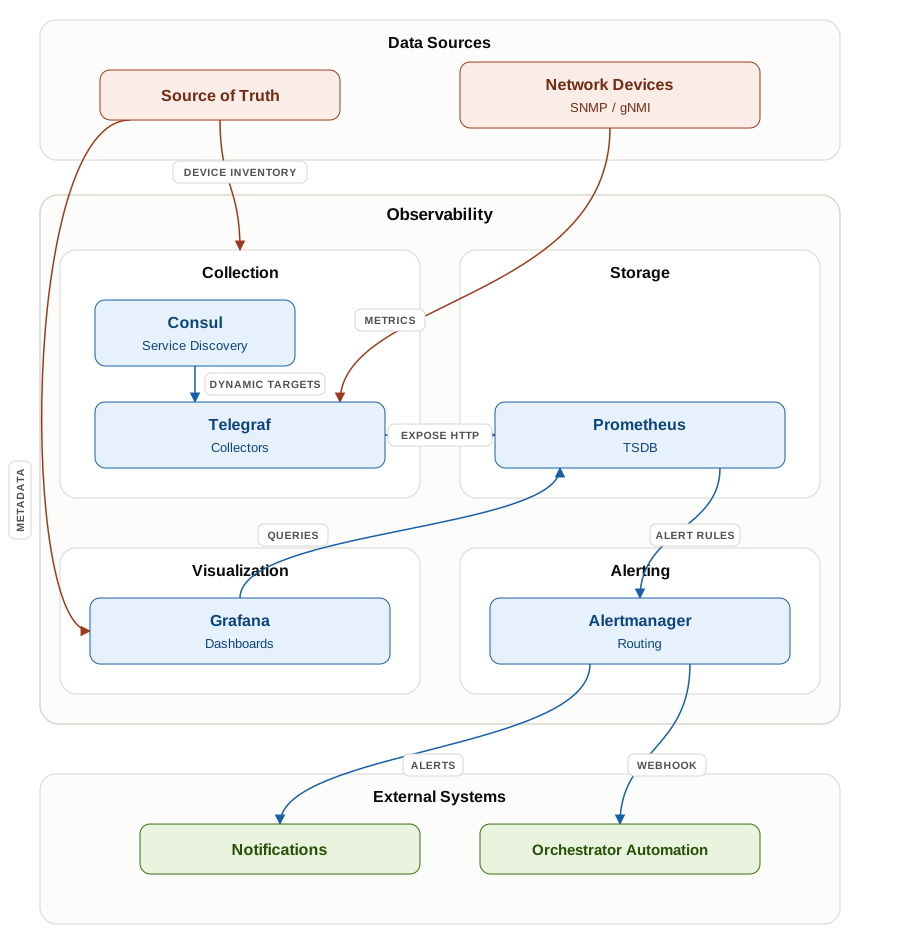
This simplistic solution architecture is covered extensively in the Modern Network Observability book. If you want a hands-on approach with a lab scenario to test, give it a try.
Implementation Flow#
The seven functionalities show up in order, each one handing off to the next:
Know the targets. The Source of Truth defines which devices to monitor, with a monitoring profile and a credential reference per device. A lightweight sync service, a script driven by webhooks, keeps a service registry current, so the Inventory functionality hands collectors a live target list instead of one somebody maintains by hand.
Collect. The Collector uses that registry for service discovery and starts polling a device as soon as it appears: SNMP on the older platforms, gNMI on the newer ones.
Normalize and enrich. The Processor converts status codes to labels, renames fields into the common model, and attaches the site, role, and service context from the SoT, then exposes the result on an HTTP endpoint for scraping.
Store. Persistence scrapes those endpoints, through the same service registry, and keeps the series for 30 days at 30-second resolution. Recording rules precompute interface utilization and bandwidth rates, which is the composed-metrics pattern from the Processor section.
Detect. Alert rules express the conditions: a VLAN missing where the SoT says it belongs, utilization above 80% for five minutes, a traffic change beyond 50%. An alert router decides where each one goes, and this is where the alert-to-action contract earns its keep: alerts labelled
automation: enabledreach the Orchestrator’s webhook as structured payloads, and everything else goes to a chat channel or a paging service by severity.Show. Visualization serves one dashboard family per audience: campus-wide bandwidth trends, top saturated interfaces, and per-device drill-down with interface heatmaps. Template variables filter by site, role, or device, and the dashboards read the metrics store for the numbers and the SoT for the metadata that gives them context.
Act. A drift alert, VLAN 412 missing from a switch where the SoT says it belongs, reaches the Orchestrator as a structured payload. The Orchestrator runs the remediation workflow: it has the Executor redeploy the VLAN to that one switch, then asks Observability to confirm the fix. That closes the loop, and Chapter 8 covers the coordination side of it.
Concretely, this example fills those functions with Nautobot as the Source of Truth, Consul as the service registry, Telegraf as the Collector and Processor, Prometheus for Persistence, Alertmanager as the alert router, and Grafana for Visualization. All of it is open source and all of it is substitutable: swap the time-series database and steps 4 through 6 change their query syntax, not their shape. Figure 7.9 above shows the same pipeline with these components in place.
Solution Summary#
Operational Benefits:
- Reduced manual monitoring effort through SoT integration
- Proactive issue detection with sub-minute latency
- Closed-loop remediation reducing MTTR from hours to minutes
- Rich context combining metrics with inventory data
Scalability Considerations:
- Current architecture handles ~800 campus switches with two or three distributed collector instances behind a service registry; adding more buildings or devices means adding more collector instances, not rearchitecting
- Persistence is sufficient at ~307K series with room to grow; a single node handles up to ~1M series before requiring federation or a distributed backend
That exercise closes the chapter: seven functionalities, one campus network, and a stack you could stand up this week.
Summary#
The fan failure in the opening story was never a missing threshold. The team had thousands. It was a source nobody collected from: line-card thermal data, available over gNMI on every chassis in the fleet and polled by nothing. Observability for automation starts from that lesson. Coverage comes from the Source of Truth, not from habit, and every functionality after it exists to turn what is collected into something a workflow or a person can act on.
Seven functionalities carry that path. Inventory reads the targets from the SoT, so a device enrolled today is observed today. The Collector speaks whatever each device offers, streaming where it can and polling where it must, and respects what observation costs the device. The Processor normalizes everything into one schema and enriches it with context, which is what makes correlation possible. Distribution decouples the stages and gives you a hot window where the full firehose is affordable. Persistence keeps time series, observed state, and configuration backups, with downsampling deciding what each retention tier answers. Alerting and Analytics compares what the network does with what the SoT says it should do, and hands the Orchestrator a structured event rather than a sentence. Visualization gives each audience its own drill-down path.
Two decisions shape the rest: whether you have the team to run a composed stack or should buy one, and how you migrate from the monitoring you already run without a gap. One blind spot outlives both. The automation platform is itself a production system, and it needs observability of its own, kept separate from the stack it watches.
Observability tells the platform what happened. Chapter 8 covers the block that decides what to do about it.
References#
- Modern Network Observability, David Flores, Christian Adell, and Josh Vanderaa (Packt, 2024). A hands-on approach to network observability using open source tools such as Telegraf, Prometheus, and Grafana; the direct practical companion to this chapter.
- Observability Engineering, Charity Majors, Liz Fong-Jones, and George Miranda (O’Reilly, 2022). The distinction between monitoring and observability and the case for high-cardinality, event-based telemetry that underpins this chapter’s data model.
- Site Reliability Engineering, Beyer, Jones, Petoff, and Murphy (O’Reilly, 2016). Monitoring, the four golden signals, and SLI/SLO design; the basis for turning raw telemetry into actionable service health. (Full text free online.)
- Network Programmability and Automation, 2nd Edition, Matt Oswalt, Christian Adell, Scott S. Lowe, and Jason Edelman (O’Reilly, 2023). Streaming telemetry, gNMI, and model-driven data collection that feed the Collector and Observability blocks.
💬 Found something to improve? Send feedback for this chapter